연구실 식구들 모두 대구수목원으로 봄나들이를 다녀왔습니다~!
연구실 식구들 모두 대구수목원으로 봄나들이를 다녀왔습니다~!
본 연구팀에서 한양대학교 조항준 교수 연구팀과 공동으로 수행한 대뇌의 기능적편측성 계산에 대한 방법론을 제시한 논문이 출판되었습니다!
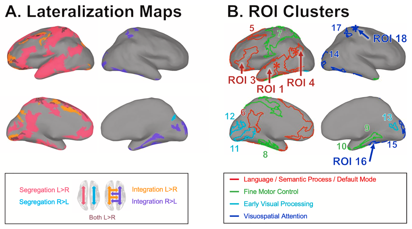
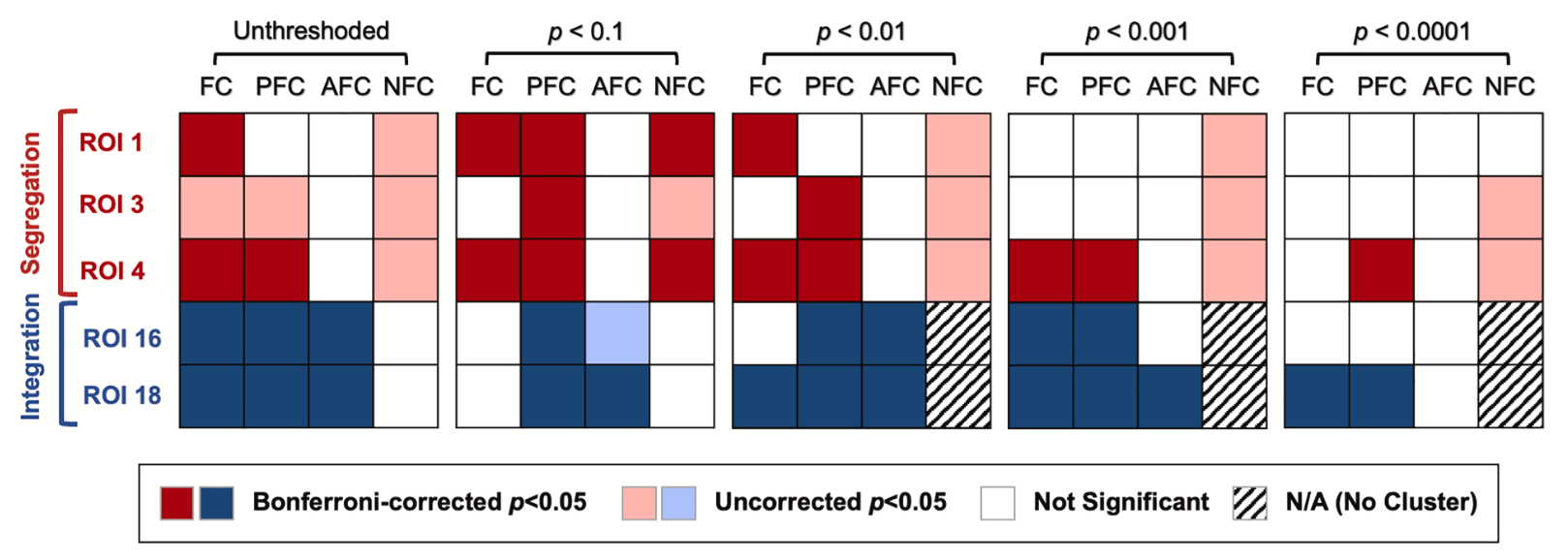
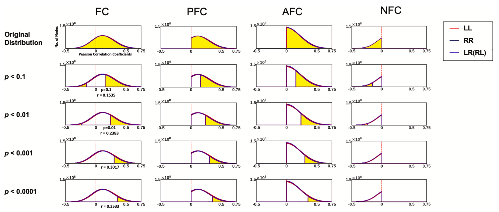
Lee T, Kim KH, Ha SY, Jo HJ. Toward a better measure of functional laterality: Comparing and refining laterality indices in resting-state functional connectivity. Neuroimage. 2026 Feb 4;328:121782. doi: 10.1016/j.neuroimage.2026.121782.
https://www.sciencedirect.com/science/article/pii/S105381192600100X?via%3Dihub
본 연구팀에서 수행한 소아청소년 발달장애환자의 장기추적조사를 통한 조현병 스펙트럼장애 발병율에 대한 역학연구결과라 출판되었습니다!
Lee T, Choi BS, Kim JH. Cumulative incidence of schizophrenia-spectrum disorders in children and adolescents with neurodevelopmental disorders: A retrospective cohort study. Psychiatry Res. 2026 Jan 27;358:116981. doi: 10.1016/j.psychres.2026.116981.
https://www.sciencedirect.com/science/article/abs/pii/S0165178126000429?via%3Dihub
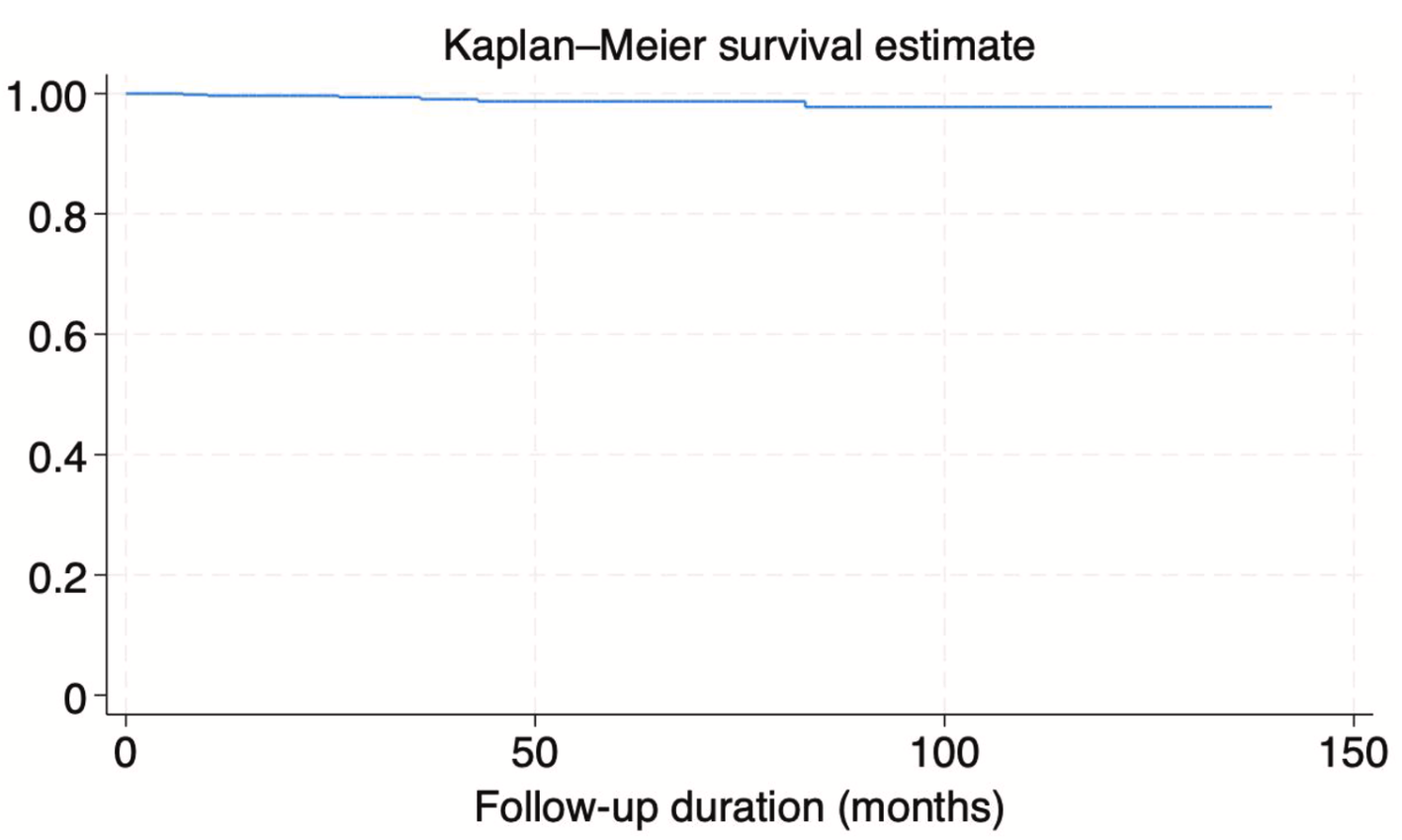
본 연구팀에서 아편계 약물 중독 환자를 대상으로 아편금단 척도 표준화 논문을 발표하였습니다.
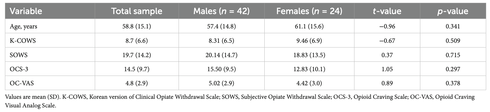
Lee TY, Im A, Ha M, Oh JY, Park KB, Kim DH, Kang HS. Validation of the Korean Version of the Clinical Opiate Withdrawal Scale. Frontiers in Public Health.;13:1706053.
https://www.frontiersin.org/journals/public-health/articles/10.3389/fpubh.2025.1706053/full
DGIST 유재석, 현정호 교수 연구팀과 함께한 초음파를 이용한 초고해상도 이미징 논문이 발표되었습니다!
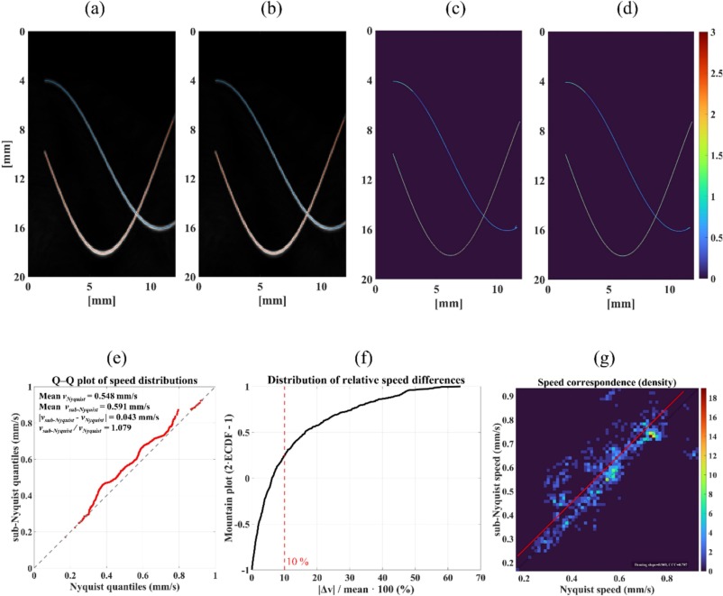
Ultrasound localization microscopy lite (ULM lite): ultrasound localization microscopy with resource-efficient signal processing scheme. Seong H, Jung J, Jung D, Guezzi N, Nam S, Lee S, Noman M, Her T, Cho E, Yoon H, Lee T, Hyun JH, Yu J. Ultrasonics. 2025 Oct 9;159:107849.
https://www.sciencedirect.com/science/article/pii/S0041624X25002860?via%3Dihub#f0030
우리 연구팀의 지역사회 조울증 고위험군 역학조사와 선별도구 BPSS-AS-P 표준화 논문이 발표되었습니다.
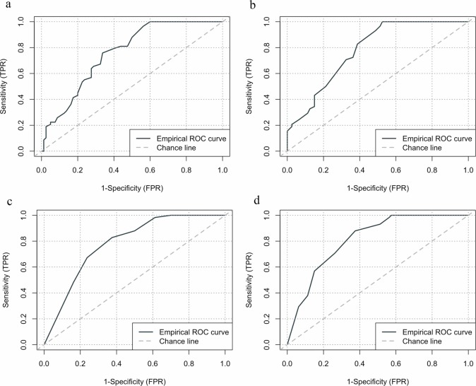
Community prevalence of at-risk state for bipolar disorder: Validation of the Korean version of Bipolar Prodrome Symptom Interview and Scale-Abbreviated Screen for Patients (BPSS-AS-P). Lee J, Lee T*, Correll CU. Asian J Psychiatry 2025 Aug, 104669
https://www.sciencedirect.com/science/article/pii/S1876201825003120#fig0015
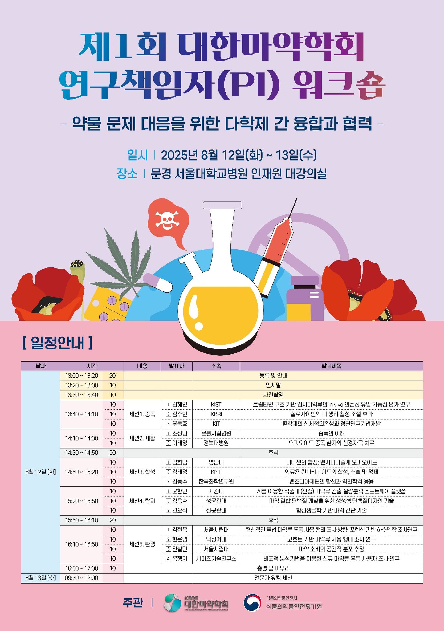
2025년 8월 12일에서 13일까지 1박2일 일정으로 서울대학교병원 인재원에서 대한마약학회 연구책임자 워크샵을 실시합니다. 이번 워크샵은 이태영 교수가 참가할 예정입니다.
우리 연구팀이 조현병과 우생학에 대한 연구가 출판되었습니다.
Lee T. Schizophrenia, Eugenics, and Stigma: The Legacy of Nazi Psychiatry and Ethical Lessons for Modern Mental Health Care. Psychoanalysis. 2025 Jul 31;36(3):49-56.
http://www.jkapa.org/journal/view.html?uid=596&&vmd=Full
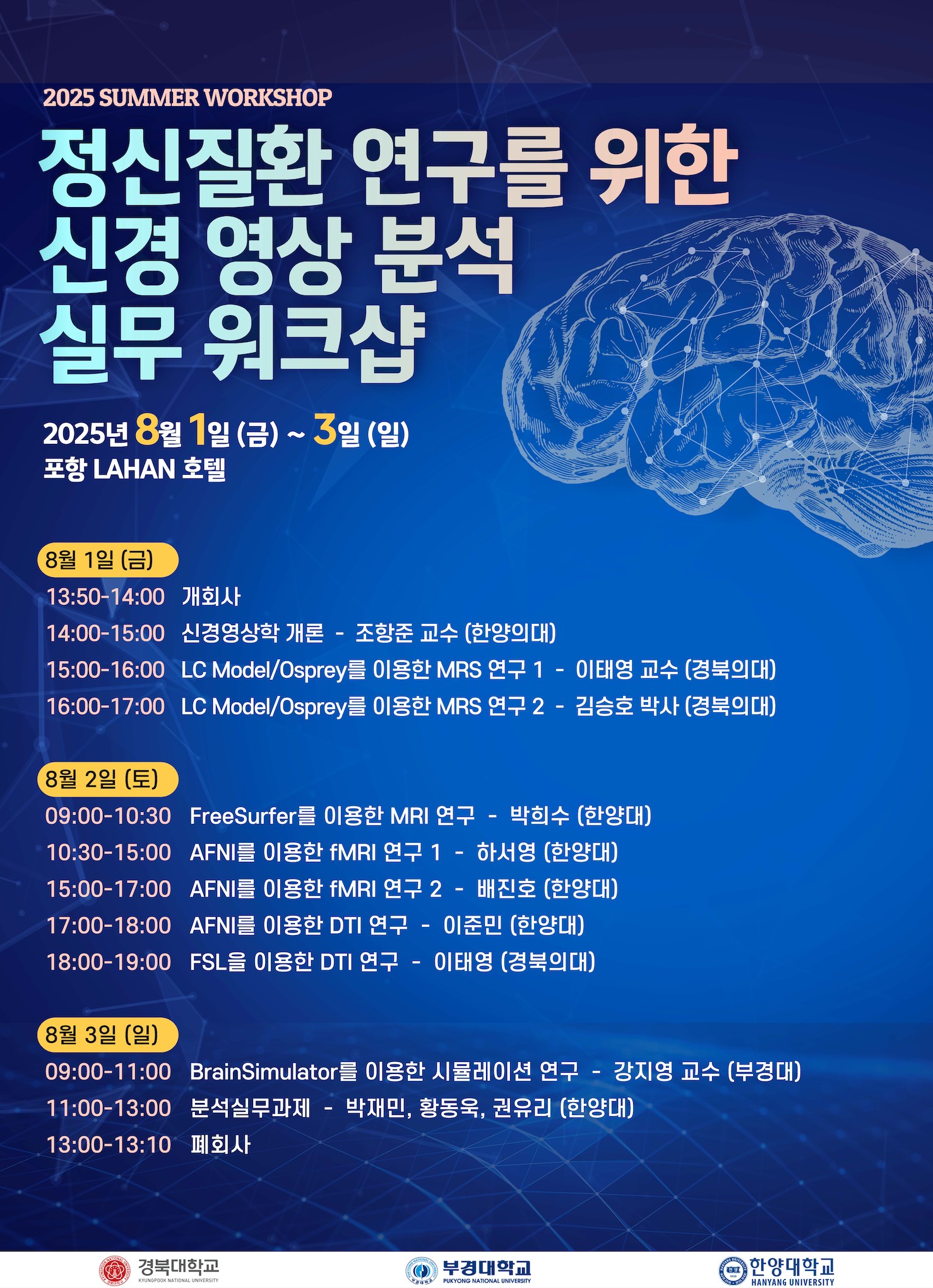
2025년 8월 1일에서 3일까지 2박3일 일정으로 포항 라한호텔에서 뇌영상분석 워크샵을 실시합니다.
이번 워크샵은 저희 연구팀과 한양대학교 조항준 교수 그리고 부경대학교 강지영 교수 연구팀이 함께할 예정입니다.
우리 연구팀이 바둑프로기사들을 대상으로 수행한 어림수 짐작의 뇌기전 연구가 출판되었습니다.

The neural basis of intuitive approximate number system in board game Go (Baduk) experts. Lee T, Jo HJ, Kim M, Kwon JS. Sci Rep. 2025 May 12;15(1):16400. doi: 10.1038/s41598-025-98605-9.